
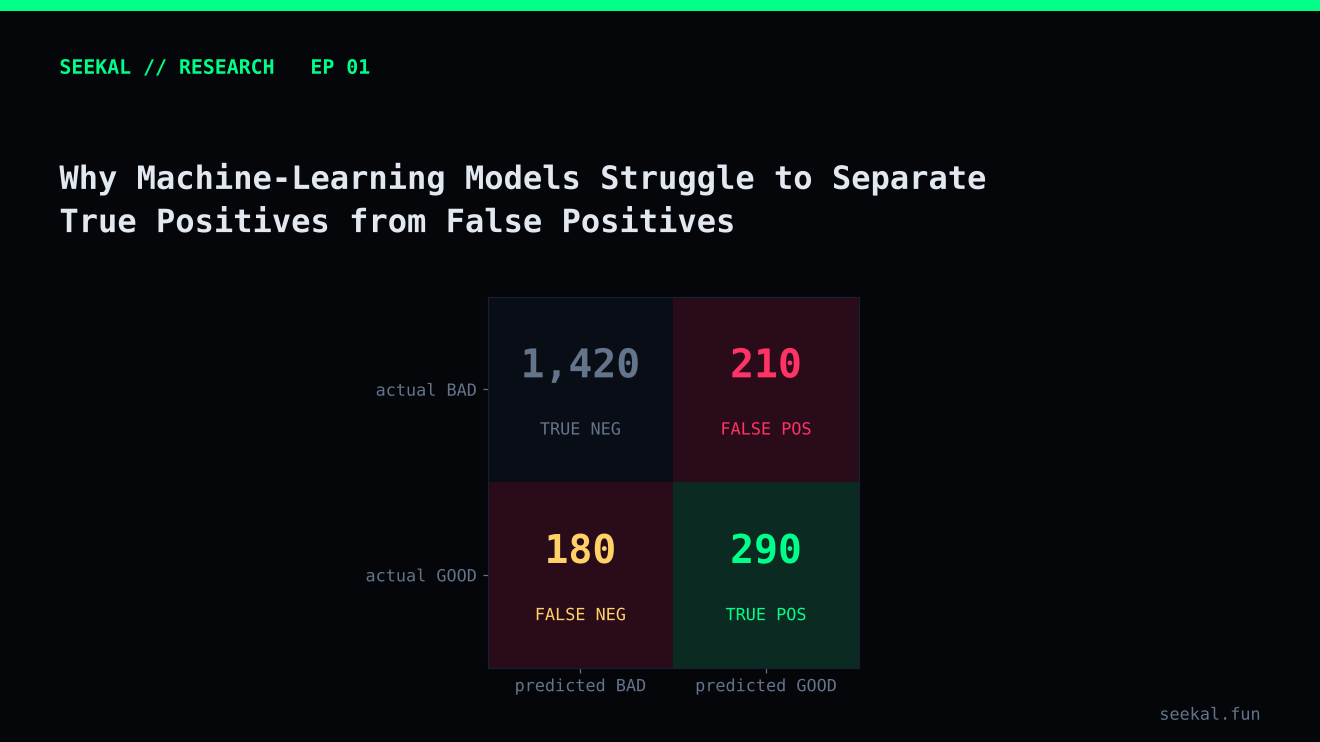
A model can look convincing in a dashboard and still make poor decisions. One reason is that a model score is not the same thing as a correct prediction. Another is that the examples a model calls promising often contain both genuine successes and false positives.
That distinction matters in any classification problem, but it becomes especially important when a label is rare and the environment changes quickly. In a token-launch dataset, most observations may not meet the chosen success definition. A model that flags many candidates can therefore produce a large number of false positives even when its overall accuracy looks respectable.
Start with the meaning of a positive
Before measuring a model, define what “positive” means. In the BSC research example used throughout this series, a token is labelled GOOD when its price reaches a fixed target multiple of the reference entry price within a set look-ahead window. Other outcomes are labelled BAD.
This is a research label, not proof that a real participant could have captured that return. The maximum may occur briefly, liquidity may be insufficient, and fees, slippage, priority costs or execution delays may change the outcome. The label is useful for studying a defined market pattern, but it must not be confused with realised profitability.
Once the definition is fixed, the four outcomes are straightforward:
- True positive: the model flags a token that meets the GOOD label.
- False positive: the model flags a token that does not meet the GOOD label.
- True negative: the model does not flag a token that is BAD.
- False negative: the model does not flag a token that would have met the GOOD label.
The model's job is not merely to produce a high score. It is to make the balance between these outcomes useful for the decision being studied.
Why false positives are so common
First, the classes may be imbalanced. The working BSC dataset contained 2,563 labelled observations, of which 656, or about 25.6%, were GOOD. A model that predicts BAD for every row would be correct roughly three-quarters of the time, yet it would identify no GOOD examples. Accuracy alone would hide that failure.
Second, features are imperfect proxies. Early volume, liquidity, buyer counts and concentration can describe activity, but none proves that demand is durable. A token can show intense early activity and still fail the chosen outcome definition. A model may learn that a pattern is associated with success without learning a reliable cause of success.
Third, the label itself contains uncertainty. A peak-price outcome can be sensitive to a single observation. If price data is noisy or the path to the peak is not realistically executable, the model can appear to identify a winner while the underlying opportunity is much less clear.
Fourth, the market is not stationary. Wallet behaviour, launch mechanics, liquidity conditions and participant strategies can change. A relationship that worked in one period may weaken in another.
What the candidate threshold revealed
In one out-of-fold evaluation of the Stage 1 BSC model, lowering the candidate threshold increased the number of selected rows but also admitted many more BAD labels. At a threshold of 0.50, the evaluation contained 657 candidates: 224 GOOD and 433 BAD, a GOOD rate of about 34.1%. At 0.65, there were 125 candidates: 54 GOOD and 71 BAD, or 43.2% GOOD. At 0.75, only 13 candidates remained, nine GOOD and four BAD.
Those figures illustrate a common trade-off: stricter selection can improve the proportion of positives while sharply reducing coverage. They are results from one historical evaluation, not a universal threshold recommendation. Small selected groups are especially uncertain; nine GOOD examples out of thirteen is encouraging evidence, but not enough to establish durable performance.
Diagnose the errors, not just the score
A useful review begins with the confusion matrix at the threshold that would actually be used. Then examine false positives one by one. Did they have high early volume but little incremental participation? Was liquidity thin? Were trades concentrated in a small number of wallets? Did a feature become extreme because its denominator was tiny? Did the data arrive late or contain a measurement issue?
Look for repeated failure modes rather than inventing a story for each token. A single false positive can be noise. A recurring pattern may reveal a feature that needs better definition, a missing interaction, a data-quality rule or a more careful label.
Also inspect false negatives. If the model misses many GOOD examples, it may be too conservative, the feature set may be incomplete, or the threshold may be misaligned with the goal. Reducing false positives at any cost can simply produce a model that rarely selects anything.
A repeatable error-review workflow
Create a review table with one row per selected observation and columns for the model score, label, launch period, key feature values and any known data-quality flags. Sort the table into true positives and false positives, then compare their distributions. Avoid reading wallet or trade histories only for the most memorable failures; that encourages confirmation bias. Use the same review rules for every case, and record hypotheses before testing them. A useful finding should be measurable—for example, “false positives are more concentrated in the lowest liquidity decile”—and then checked on a later period.
The practical lesson
False positives are not a sign that machine learning is useless. They are evidence about the limits of the current features, labels, sample and validation design. The right response is to measure them, classify their patterns and test changes on data the model did not use to learn those changes.
A credible model report should state the positive definition, the number of selected observations, true and false positives, precision, recall, the evaluation period and the uncertainty created by sample size. It should also distinguish a research label from an executable outcome.
Prediction is only the beginning. The quality of the work is determined by how honestly the errors are measured and how carefully each proposed improvement is tested.
Research note: The dataset counts and threshold examples in this article come from one BSC research run described in the project notes. They are historical, dataset-specific observations and should be recalculated before publication if the dataset or pipeline changes.