
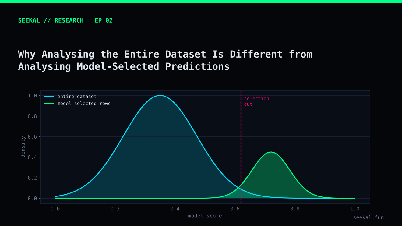
A feature can look useful across an entire dataset and become much less useful among the rows a model actually selects. The reverse can also happen: a feature with a weak overall relationship to the label may help distinguish the strongest candidates inside a selected group.
This is one of the most important shifts in model analysis. The question is not only “Which features are associated with GOOD outcomes?” It is also “Among the observations that pass the first model, which features help separate the better candidates from the weaker ones?” Those are different statistical questions.
The population changes after selection
Imagine a dataset containing every token in a research period. It includes quiet launches, highly active launches, very low-liquidity launches and everything in between. A Stage 1 model evaluates all eligible rows and assigns a score. A threshold then selects a subset.
That subset is not a random sample of the original dataset. It is a population created by the model's decision rule. The rows may have similar Stage 1 scores, stronger early activity or a particular combination of features. Relationships measured in the full dataset do not automatically carry over unchanged.
For example, early volume may distinguish GOOD from BAD across all launches. But after Stage 1 has already selected rows with relatively strong early volume, there may be little remaining variation in that feature. Within the candidate group, buyer distribution or liquidity development could become more informative.
A two-stage example
In the BSC project, Stage 1 was used to identify candidates. A second model was then tested to evaluate candidates using additional information, including liquidity, buyer concentration, early selling and volume-quality measures.
The purpose of Stage 2 was not to pretend that the whole market had become easier to predict. It was to ask a narrower question: given that Stage 1 has already selected this candidate, can the second model rank or filter candidates more effectively?
This design changes the target population. Stage 2 should be trained and evaluated on candidates selected by a Stage 1 model that did not use their eventual labels to make those selections. That is why out-of-fold Stage 1 predictions are essential. If Stage 2 receives in-sample Stage 1 scores, it may learn from an unrealistically favourable version of the first model.
Selection can create misleading relationships
Selection can also distort correlations. Suppose Stage 1 selects tokens partly because of high volume and partly because of liquidity. Within the selected group, a token with less volume may have needed stronger liquidity to cross the threshold. Volume and liquidity can therefore appear related inside the selected group even if their relationship in the full dataset is different.
This is a form of selection bias. In more technical settings, conditioning on a variable influenced by multiple factors can create or strengthen associations among those factors. The practical implication is simple: do not assume that a relationship observed among model-selected rows is a causal relationship or that it will hold in the full population.
Compare like with like
A sound analysis should report at least two views. The first examines feature distributions and label rates across the full eligible dataset. The second examines the same quantities among model-selected candidates. Keep the time period, feature definitions and label rules consistent so the difference is interpretable.
For each view, show sample size. A quartile containing 500 rows is not comparable in uncertainty to a bucket containing 12 rows. Also show the number of GOOD and BAD observations, not only percentages. A high GOOD rate in a tiny bucket may be a fragile result.
When the goal is a second-stage model, build the Stage 2 training table from out-of-fold Stage 1 predictions. Respect chronology: the first model must be trained only on earlier data when it scores a later fold. Apply a purge interval where labels overlap future outcome windows.
What the BSC experiment teaches
The Stage 1 candidate table showed a clear coverage-versus-quality trade-off. In one evaluation, a 0.50 threshold produced 657 candidates with a GOOD rate of about 34.1%, while a 0.65 threshold produced 125 candidates with a GOOD rate of about 43.2%. This tells us what the selected population looks like at those thresholds; it does not tell us which features will be most useful within that population.
The later Stage 2 tests evaluated a smaller candidate population. Their results were mixed across cross-validation and the final chronological holdout, which is a reminder that an apparent improvement within a selected group still needs independent validation.
Keep population definitions in every report
A good report names the population in the title of each chart or table. “Full-dataset GOOD rate” and “Stage 1 candidate GOOD rate” are clearer than a generic “GOOD rate”. Include the date range and the selection rule beside the figure. When the candidate threshold changes, the population changes too, so do not compare feature distributions from two thresholds as if they were identical groups. If you compare thresholds, show how many rows enter and leave the candidate pool and how the class balance changes.
The practical lesson
Always state which population a statistic describes: the complete dataset, a candidate pool, a cross-validation fold or a final holdout. Avoid moving a conclusion from one population to another without testing it.
A model-selected dataset is not simply a smaller copy of the original dataset. It is a different analytical setting, with its own class balance, feature ranges, biases and uncertainty. Understanding that distinction is essential when building cascaded models, filters or ranking systems.