
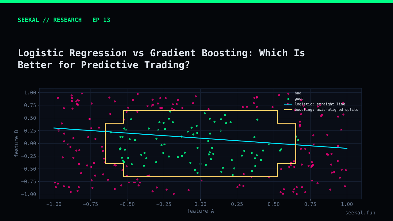
When comparing algorithms, it is tempting to ask which one is best. A more useful question is: which model is better suited to this dataset, this validation design and this decision? Logistic regression and gradient boosting make different assumptions, offer different kinds of flexibility and fail in different ways.
Neither should be selected because it is fashionable or because it won one small test.
Logistic regression: a disciplined baseline
Logistic regression estimates the probability of a binary outcome using a linear combination of features passed through a logistic function. Its default structure is additive on the log-odds scale. It does not automatically discover every nonlinear relationship or interaction.
That limitation can be an advantage. A regularised logistic model is relatively simple, quick to train and easier to inspect than a large ensemble. Standardised coefficients can offer a view of conditional associations, although correlated features make individual coefficients difficult to interpret.
Regularisation penalises large coefficients and can reduce overfitting. It does not make the model immune to leakage, poor labels, missing nonlinearities or unstable data.
Gradient boosting: flexible decision structure
Gradient boosting builds an ensemble of decision trees sequentially. Each new tree attempts to improve the errors of the existing ensemble. The model can represent nonlinear relationships and interactions without requiring every interaction to be manually specified.
That flexibility can be valuable when the relationship between volume, liquidity and participation is conditional. But it creates more tuning choices. With a small dataset, a flexible model may learn patterns that do not repeat. Results can be sensitive to learning rate, number of leaves, tree count, minimum leaf size and regularisation.
Feature importance also needs caution. When features are correlated, the model may distribute importance among substitutes. A ranking from one fitted model is not a causal explanation.
What happened in the BSC Stage 2 comparison
The project tested a regularised logistic model and a LightGBM model on a Stage 2 candidate dataset. In one chronological holdout of 112 candidates, logistic regression achieved ROC-AUC 0.6242 and PR-AUC 0.4674. LightGBM achieved ROC-AUC 0.5890 and PR-AUC 0.4705.
At a probability threshold of 0.50, both models selected 46 candidates. Logistic regression selected 22 GOOD and 24 BAD, giving 47.83% precision and 56.41% recall. LightGBM selected 17 GOOD and 29 BAD, giving 36.96% precision and 43.59% recall.
Cross-validation did not produce a simple universal verdict. Pooled average precision was 0.3947 for logistic regression and 0.4275 for LightGBM; mean fold average precision was 0.4159 and 0.4119 respectively. The ranking metrics and holdout results were mixed.
The sample is not large enough to conclude that logistic regression is the better algorithm in general. The reasonable interpretation is that logistic regression was stronger on several measures in this particular holdout, while the broader evidence remains inconclusive.
Compare the models fairly
Both models should receive the same eligible candidates, feature definitions, chronological folds and purge rules. Tune only within development data. Use a consistent metric plan and compare not only AUC but also precision, recall, selected count, calibration and stability by period.
For a practical prediction system, also consider data availability, model latency, monitoring and the cost of maintaining the feature pipeline. An extra point of offline metric performance may not justify a much more fragile system.
Compare the cost of complexity as well as the score
The model comparison should include implementation details that affect reliability: prediction latency, missing-data behaviour, ease of recalibration, sensitivity to feature drift and the effort required to reproduce training. A small metric difference may not justify a more complex pipeline if its performance is unstable or its inputs are difficult to obtain consistently. Conversely, if nonlinear interactions repeat across periods and materially improve the chosen objective, the additional flexibility may be justified.
The practical lesson
Logistic regression offers a disciplined, regularised baseline. Gradient boosting offers nonlinear and interaction capacity. Test both under the same chronological design, report all relevant metrics and avoid declaring a winner from one small holdout. The right model is the one whose performance and behaviour remain credible on later data.