
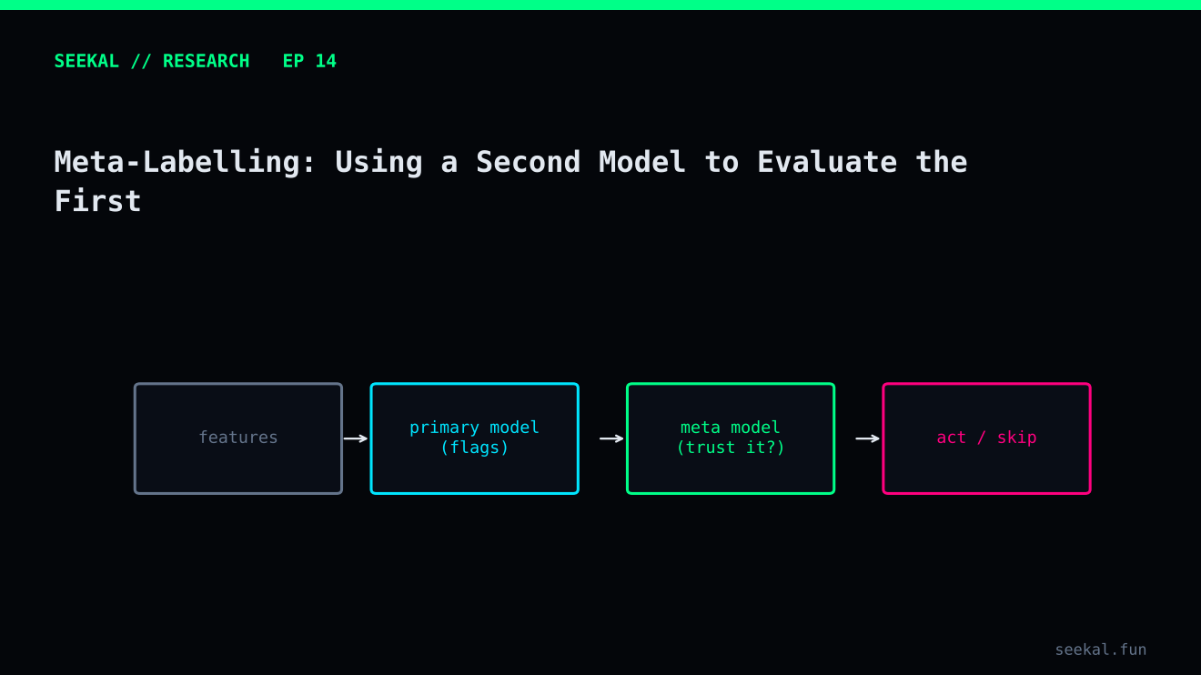
A first-stage model can be useful at finding a broad set of candidates without being precise enough for a narrower decision. Meta-labelling adds a second model that evaluates the cases selected by the first. The goal is not to replace the original model automatically; it is to learn whether additional information can improve the assessment of its selected cases.
This approach is attractive when the first model has useful recall but produces too many false positives. It is also easy to implement incorrectly.
The two-stage idea
Stage 1 scores the full eligible population. A threshold turns those scores into a candidate set. Stage 2 receives only candidates and uses additional information or a different representation to estimate whether the candidate meets the positive label.
The two stages answer different questions. Stage 1 asks, “Which observations are worth examining?” Stage 2 asks, “Among those observations, which are more likely to meet the outcome definition?”
The second stage cannot recover candidates that Stage 1 never selected. Its maximum possible recall is therefore constrained by Stage 1's coverage. This should be visible in the evaluation report.
The leakage problem
The most important requirement is honest Stage 1 predictions for Stage 2 training data. If the first model scores a row after having trained on that same row, its score is an in-sample prediction. It is usually more optimistic than a score on a truly unseen observation.
Instead, generate out-of-fold scores. For each training fold, fit Stage 1 on earlier eligible data and score a later fold that was not used in fitting. With time-dependent labels, preserve chronology and purge observations whose future outcome windows overlap the validation boundary.
Then construct the Stage 2 training table from those out-of-fold candidate predictions. The final Stage 1 model can be fitted on the development period and applied to a later untouched holdout; Stage 2 must also remain blind to the holdout labels until the final evaluation.
What the BSC experiment showed
The BSC project evaluated Stage 2 logistic regression and LightGBM on candidates selected by the first-stage model. In one final chronological holdout, 112 candidates were available. Logistic regression achieved ROC-AUC 0.6242 and PR-AUC 0.4674; LightGBM achieved 0.5890 and 0.4705.
At the 0.50 Stage 2 probability threshold, each model selected 46 candidates. Logistic regression identified 22 GOOD and 24 BAD, while LightGBM identified 17 GOOD and 29 BAD. The original Stage 1 threshold of 0.75 selected five cases in that holdout, all five GOOD. The Stage 2 approaches expanded the selected set, adding both positive and negative cases.
This comparison illustrates the trade-off: the second stage can increase coverage, but the added candidates include false positives. The five-of-five Stage 1 result is too small to establish a stable benchmark, and the mixed Stage 2 metrics do not prove that either second-stage model is production-ready.
Evaluate the whole cascade
Do not report Stage 2 in isolation. Evaluate the end-to-end system from the original population. Include the number of all eligible rows, Stage 1 candidate count, Stage 2 selected count, true and false positives, false negatives and the label prevalence at each stage.
Report the performance at several Stage 1 thresholds. A stricter first stage may produce a smaller, cleaner candidate pool but limit the recall available to Stage 2. A looser first stage may give Stage 2 more opportunities but increase its workload and change its class balance.
Also compare against a Stage 1-only baseline on the same chronological holdout. If the cascade does not improve the decision-relevant measures consistently, its extra complexity may not be justified.
Measure the value added by Stage 2
Compare three outputs on the same later period: the full Stage 1 candidate set, the Stage 2 selected set and a simple baseline ranking that uses no second-stage model. This reveals whether Stage 2 adds value beyond merely changing the threshold or sorting by the Stage 1 score. Report both the number of GOOD cases retained and the number of BAD cases introduced. A second model is useful only when its improvement is repeatable and large enough to justify the additional pipeline and monitoring burden.
The practical lesson
Meta-labelling is a conditional second opinion, not a magic correction layer. Use out-of-fold first-stage scores, preserve time order, evaluate the complete cascade and keep a genuinely untouched final period. The second model earns its place only when it improves the system on later data.