
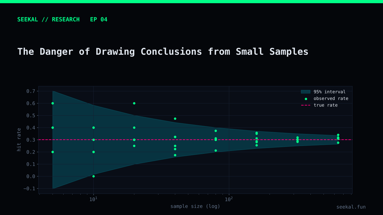
A result can be mathematically correct and still be a weak basis for a decision. If a model selects five cases and all five are positive, the observed precision is 100%. But five observations do not establish that the model's true precision is 100%, or even close to it.
Small samples create uncertainty. The smaller the sample, the more easily a few observations can change a percentage, a ranking or a model comparison.
Percentages hide the denominator
Consider two results:
- 9 positives among 13 selected cases: 69.2% precision.
- 90 positives among 130 selected cases: 69.2% precision.
The observed percentages are identical. The evidence is not equally strong. The second result is based on ten times as many observations and is generally less sensitive to one case changing category.
That is why every percentage should be accompanied by its numerator and denominator. “69% precision” is not a complete report. “9 of 13 selected cases were positive” tells the reader how much evidence supports the estimate.
A small threshold group can look exceptional
In one BSC Stage 1 out-of-fold evaluation, the 0.75 threshold produced 13 candidates, nine GOOD and four BAD. That is a GOOD rate of about 69.2%. At first glance, the rate looks attractive. But the sample is small: changing the outcome of one candidate moves the rate by about 7.7 percentage points.
In a later Stage 2 chronological holdout, the original Stage 1 threshold selected only five candidates, all of which met the research GOOD label. That is a useful observation, but it is far too small to establish stable precision. A handful of cases can be affected by unusual market conditions, data quirks or chance.
Do not dismiss small results. Treat them as signals that deserve more evidence, not as proof.
Confidence intervals make uncertainty visible
A confidence interval gives a range of values compatible with the observed data under a stated statistical procedure. For a binomial proportion such as precision, Wilson or exact intervals are often more appropriate than a simple normal approximation, especially for small samples or proportions near zero or one.
The interval does not guarantee that the true value lies inside it. It communicates how uncertain the estimate is under the model's assumptions. If selected observations are dependent, clustered by launch period or otherwise non-independent, a simple binomial interval may still understate uncertainty. The validation design matters.
Repeated experimentation creates another trap
Suppose a researcher tries 50 thresholds, 20 feature combinations and 10 model settings, then reports the best-performing result. Even if every experiment is individually reasonable, searching many configurations makes it more likely that one looks unusually good by chance.
This is a form of multiple-comparison or selection bias in the research process. The chosen configuration has benefited from being selected because it performed well on the data used to compare candidates. Its apparent performance may not repeat.
Keep a record of all experiments, define a primary metric before comparing models, limit tuning to development data and reserve a later untouched period for final evaluation. Once the holdout has influenced design decisions, it is no longer an untouched holdout.
Time matters as much as row count
A dataset with 500 launches from one short market regime may provide less evidence of generalisation than a dataset with 500 launches spread across several distinct periods. Samples close together in time can share market conditions, participants and data-generation patterns.
Chronological validation helps reveal this. Report performance by fold or period, not only as one pooled number. Large differences between periods may indicate regime sensitivity.
A practical small-sample checklist
Whenever a result looks unusually strong, ask: how many observations are behind it? How many positive and negative labels? How many separate time periods? Was the threshold selected on the same data? Were many alternatives tested? Are observations independent? Does the positive label reflect the real outcome of interest?
If the answer reveals limited evidence, write the conclusion accordingly: “promising in this small sample,” “requires more chronological validation,” or “not yet conclusive.” This is stronger research communication than pretending uncertainty does not exist.
Make sample size visible in visualisations
Use labels such as “9/13” directly on charts instead of displaying 69% alone. When possible, include an uncertainty interval and avoid ranking groups whose intervals are extremely wide. If a fold contains very few positive cases, report the fold rather than hiding it, but state that its estimate is unstable. Do not merge periods simply to create a larger number unless the periods are genuinely comparable. More rows are useful only when they represent the population and conditions the model is expected to face.
The practical lesson
A small sample is not useless; it is simply easy to overinterpret. Keep counts beside percentages, show uncertainty, repeat tests over later periods and resist choosing a model because one small holdout happened to favour it. Trust grows when limitations are visible.