
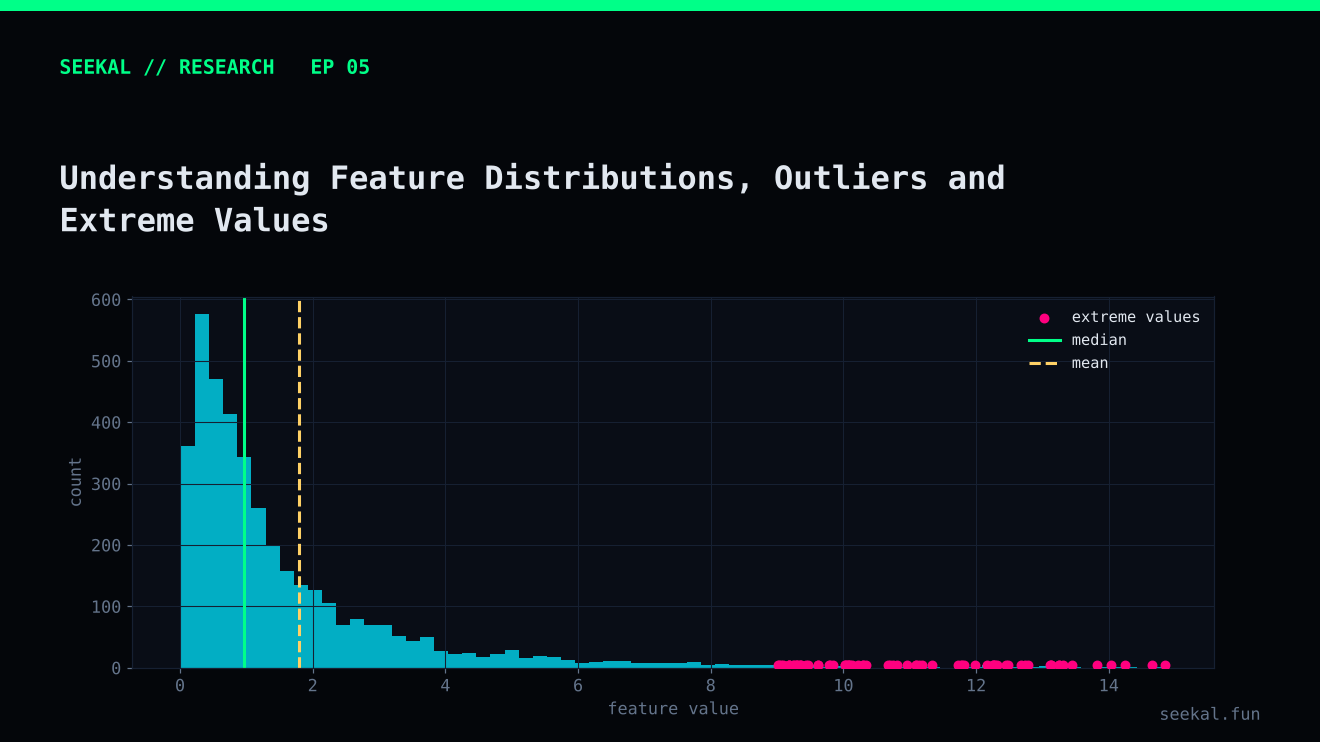
Machine-learning models do not receive the world as it is. They receive columns of numbers created by data pipelines. Those numbers may be skewed, sparse, rounded, duplicated, truncated or affected by unusual events. Before changing a model because a feature appears powerful, understand how that feature is distributed and how it was calculated.
An extreme value can represent a genuine rare event. It can also be a measurement error, a small-denominator effect or a feature-definition problem. The point of outlier analysis is not to delete every unusual observation. It is to learn what produced it.
Look beyond the average
For each numerical feature, examine the count of valid values, missingness, minimum, maximum, median, standard deviation and selected percentiles. The 95th, 99th and 99.9th percentiles are particularly useful for heavy-tailed features because the maximum alone tells little about how unusual an observation is.
Plot the distribution on both linear and logarithmic scales where appropriate. A histogram can show whether most observations are concentrated near zero while a small number stretch the axis. A box plot can flag extreme tails, but it cannot explain why they exist.
Compare distributions by label as well. The overall distribution can conceal the fact that GOOD and BAD observations have different tails or different relationships with the feature.
Inspect the feature-generation logic
A model sees the final column, not the intention behind it. Trace an extreme value back through the pipeline. Check units, scaling, rounding, time windows, missing-value handling, zero denominators and whether values are cumulative or incremental.
In the BSC pipeline, for example, growth_10 was calculated as cumulative vol_10 divided by cumulative vol_5, after the volume values had been rounded. That formula has a specific interpretation and can produce extreme ratios when the five-minute denominator is very small. A very high value is not automatically evidence of extraordinary demand.
One token in the research review had a reported growth_10 value of 20,975.2 and an observed early trade under one dollar during its first nine minutes. That observation is a reason to inspect the exact vol_5 and vol_10 inputs, not a reason to assume the record is wrong or to delete it. The ratio's denominator must be confirmed from the source rows.
Separate rare behaviour from bad data
A genuine outlier may be exactly the behaviour the model should learn about. Removing it simply because it is unusual can erase important information. Conversely, retaining a corrupted value can distort scaling, feature importance or split decisions.
For every extreme record, check:
- Does the raw source data support the value?
- Is the time window correct?
- Are the units consistent?
- Does the formula behave sensibly near zero?
- Is the observation a legitimate rare case or a pipeline defect?
Document the decision. If the value is valid, retain it and consider whether the model can handle the skew. If it is invalid, correct the source or apply a documented quality rule. Avoid silent clipping that changes the research population without explanation.
Transformations and robust alternatives
For positive, strongly skewed variables, a logarithmic transformation can reduce the influence of the far tail. A common form is log1p(x), which is defined at zero. Ratios may need separate treatment because a log transformation does not solve an unstable denominator. Winsorisation or clipping can limit extreme values, but thresholds must be fitted on training data only and validated chronologically.
Tree-based models can tolerate some nonlinear scaling differences, but they are not immune to corrupt features, leakage or misleading ratios. Linear models often benefit from standardisation, while still requiring careful treatment of skew and outliers.
Build an outlier audit trail
For each investigated extreme, save the token identifier internally, raw trade rows, derived numerator and denominator, time-window boundaries, calculation version and final disposition. A separate audit file prevents a future pipeline change from making the original decision impossible to reconstruct. Re-run the same audit after changes to rounding, quote conversion or event timing. This is especially important when an extreme observation could materially affect a percentile, a feature transformation or a model split.
The practical lesson
Outlier analysis is a feature-engineering audit, not a cosmetic cleaning step. Inspect percentiles, compare labels, trace extreme rows to raw inputs and document every transformation. Keep the distinction between “unusual but valid” and “invalid measurement” clear. A model becomes more reliable when its inputs have understandable meanings.