
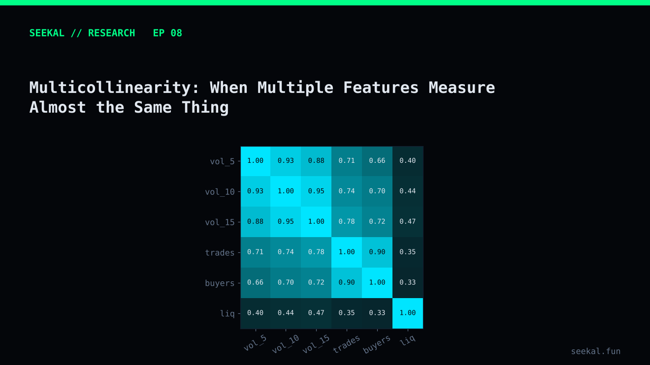
A dataset can contain dozens of features and still describe only a handful of underlying behaviours. Several columns may be different versions of the same measurement: cumulative volume over adjacent windows, liquidity at related timestamps, or multiple concentration statistics.
This overlap is called multicollinearity. It does not always make a model inaccurate, but it can make interpretation unstable and can encourage researchers to mistake duplicated information for many independent signals.
What multicollinearity means
In a linear model, multicollinearity occurs when one feature can be approximated by a combination of other features. If two columns are almost identical, the model has difficulty assigning a unique contribution to each one.
For example, vol_10 includes the volume measured in vol_5. The two are mechanically related. The incremental amount from minute five to minute ten is also derived from them. Adding all three may be useful for representing total scale and later activity, but the features are not independent measurements.
Other potential overlaps include:
- A percentage and its underlying count when the denominator varies little.
- Multiple top-wallet concentration measures.
- Cumulative volume and growth ratios derived from the same windows.
- Liquidity level and liquidity change where one is directly used to calculate the other.
Why it matters for different models
In ordinary linear regression, highly correlated predictors can make coefficients unstable. Small changes in the data may produce large changes in coefficient size or sign, even if predictions remain similar. Standard errors can increase, making individual coefficients harder to interpret.
Regularisation can reduce coefficient instability by penalising overly large weights. Ridge-style regularisation shrinks correlated coefficients, while L1 regularisation may drive some coefficients to zero. Neither method identifies a single “true” feature when multiple columns carry nearly the same information.
Tree-based models such as gradient boosting are less sensitive to multicollinearity in some predictive settings, but feature importance can be divided among correlated variables. A feature may appear unimportant because another similar feature is chosen for a split. Importance rankings should therefore be interpreted as model-dependent evidence, not a definitive ranking of real-world causes.
How to investigate overlap
Start with a correlation matrix for numerical features. Pearson correlation measures linear association; Spearman correlation can reveal monotonic relationships that are not linear. Neither detects every form of redundancy.
Then inspect the feature formulas. A correlation of 0.95 may be less informative than discovering that one column is literally calculated from another. Build groups based on shared source data and time windows.
For linear models, variance inflation factors can help identify severe linear dependence, although they can become difficult to interpret in large feature sets and do not prove that a feature should be removed.
The most useful test is often ablation. Train a baseline, remove one feature or a coherent group, and compare out-of-time performance. If removing one column changes nothing, it may be redundant. If removing a group hurts performance, the group may carry useful information even if its internal coefficients are unstable.
A caution about coefficient interpretation
In the BSC Stage 2 logistic experiment, standardised coefficients showed positive and negative weights for features such as incremental volume, growth_10, liquidity and buyer concentration. Those coefficients describe conditional relationships given the other features included in that particular model. Because several inputs are related, a coefficient's sign or magnitude should not be treated as a standalone causal statement.
A positive coefficient for incremental volume alongside a negative coefficient for a related growth ratio does not necessarily mean that one behaviour is good and the other is bad. It may mean the model is distinguishing absolute scale from relative change, or it may reflect overlap among the predictors. The correct response is to test coherent feature groups and inspect stability across folds.
Practical ways to simplify
Group features by concept: volume scale, volume change, liquidity level, liquidity change, buyer participation, concentration and selling pressure. Compare each group against a baseline. Keep the features that improve validation performance or interpretability. Prefer a simpler representation when performance is effectively unchanged.
Do not remove features solely because their correlation is high. Two correlated features can still provide complementary information, especially when they represent different aspects of behaviour. The decision should be based on the feature definitions, the model type and chronological validation.
Look for redundancy at the formula level
A correlation heatmap is a starting point, not a full audit. Build a feature dictionary that records each feature’s source columns, time window, formula and unit. Features derived from the same raw components should be grouped for review even if their sample correlation is not extremely high. Conversely, a high correlation does not automatically mean one feature should be removed. Keep the representation that improves out-of-time performance, clarity or operational reliability.
The practical lesson
More columns do not necessarily mean more independent information. Audit formulas, inspect correlations, use ablation and interpret coefficients conditionally. A compact feature set that is stable across periods is often more valuable than a large collection of overlapping variables.