
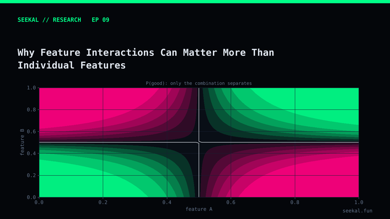
A feature can be useful only under certain conditions. High volume may mean something different when liquidity is thin than when liquidity is deep. A large growth ratio may be more informative when the starting volume is meaningful. Buyer concentration may matter differently when the number of buyers is high.
These conditional relationships are called feature interactions. They explain why evaluating each feature in isolation can miss important structure.
What is an interaction?
An interaction exists when the relationship between one feature and the outcome depends on the value of another feature.
Suppose volume is associated with positive outcomes only when liquidity is above a certain level. Looking at volume alone may show a weak or inconsistent relationship. Looking at liquidity alone may also show a weak relationship. But the combination—high volume with adequate liquidity—may be more informative.
A simple linear model can represent an interaction by adding a product term:
Here, the effect associated with x1 changes depending on x2. The interaction coefficient is not a causal explanation; it describes a pattern in the fitted model.
Examples from token-activity features
Volume and liquidity: high trading volume with low liquidity may describe a very different environment from high volume supported by deeper liquidity.
Growth ratio and starting volume: a large growth_10 ratio can be caused by a tiny vol_5 denominator. The same ratio may have a different interpretation when the baseline volume is larger.
Buyer count and concentration: many unique buyers may sound positive, but if one wallet accounts for a large share of activity, the overall participation pattern is still concentrated.
Early selling and buyer composition: a high early-seller share may be more concerning when a small number of wallets dominate buying, while its relationship may differ in a broader participation pattern.
These are hypotheses to test, not rules to assume. The meaning of a feature combination must be evaluated against the labels and then checked on later periods.
How different models learn interactions
Decision trees naturally create conditional rules. A tree might first split on liquidity and then split on volume inside one branch. Gradient boosting combines many such trees, allowing it to model nonlinear relationships and interactions without manually specifying every product term.
Logistic regression is additive unless interaction terms or nonlinear transformations are included. Its simplicity can be an advantage when the dataset is small, but it may miss conditional patterns unless they are explicitly engineered.
This creates a familiar trade-off. A more flexible model may discover complex interactions, but it can also learn noise—especially when there are few examples in each combination. A simpler model may be more stable but underfit the relationship.
Test interactions without creating a fishing expedition
Begin with a small number of domain-motivated hypotheses. For each one, inspect a two-dimensional table or plot. Use quantile buckets carefully and report the counts in every cell. Empty or tiny cells cannot support a strong conclusion.
Then compare a baseline model with a version that adds the interaction. Use chronological folds and keep all feature construction inside the training process where it depends on fitted statistics. Do not choose an interaction because it improves the final holdout and then continue reporting that holdout as an independent test.
For tree models, feature importance alone may not explain an interaction. Partial dependence or other model-interpretation tools can help, but they can be misleading when features are correlated. Always compare explanations with the actual feature formulas and observed data ranges.
Require enough observations in every interaction region
A two-dimensional plot can create many cells with very few observations. Before interpreting a high GOOD rate in one corner, check the number of cases and labels in that region. Consider coarser bins when the dataset is small, and avoid repeatedly changing bin boundaries until a desired pattern appears. If a tree model discovers a split, verify that similar split behaviour appears across folds. An interaction is more credible when it survives small changes in the sample and time period.
The practical lesson
Individual features describe dimensions of activity. Interactions describe how those dimensions work together. Look for combinations with a clear rationale, inspect the sample size in each region and test them chronologically. A complex interaction is useful only when it repeats beyond the data that inspired it.